Player Tracking in Squash with Computer Vision and Deep Learning

Implementing pose estimation algorithms to generate analytics on squash matches

For our final project at Metis, we were given carte blanche to explore any data science topic that we were interested in. I decided to use data science to explore one of my favorite sports: squash. I played throughout college and was team captain as a senior, but there are plenty of things I am missing in my game. I thought I would use data science to help better understand court positioning, and hopefully put something together that could be used by coaches at all levels of the game, as long as they had access to a camera.

The Model

The most important part of a computer project centered around person detection is using an algorithm that can accurately detect people, which is obvious but if you can’t find people with your model then you can’t do anything else. I decided to use an algorithm called DeepPose, which was originally discussed by two Google researchers in the paper I linked. The algorithm uses a Convolutional Neural Network (CNN) to predict where 17 different joints are in an image. It’s a fairly complex model, so I decided to use a pre-trained model as training my own to an acceptable level of accuracy would’ve taken me over 100 days on my local machine.

The general idea behind a CNN is to use a series of convolutional layers in order to find patterns at varying levels of an image. Convolutional layers use different image kernels convolved with an image in order to do things such as detect edges and blur images until the underlying patterns emerge. To think of it in simpler terms, you are training a computer to recognize things like the shape of a knee cap or common contours of a leg leading to a knee joint that we as humans already understand how to do. Interestingly, convultional layers are actually inspired by the organization of an animal’s visual cortex. The activation of each of these layers is ReLU (Rectified Linear Units), which is f(x)=max(0,x): setting all negative values to zero. This gives the system an aspect of nonlinearity, as all of the convolutional layers are simply linear algebra operations. ReLU is chosen as opposed to other more complex nonlinear activation functions like sigmoid of tanh because of the relative speed, which is important when dealing with matrices corresponding to images.

After the convolutional layers, there are pooling layers, which take the outputs of all of the neurons from a convolutional layer and pool them into one neuron. What this layer does is simplifies or downsamples the convolutional layer. Effectively this means that the weight of parameters is reduced, which lessens computation cost and limits overfitting. In addition, it reorganizes the filters that have been found with the convolutional layers so that the network will look more for relative positioning of elements, rather than absolute positions. It is not uncommon to also include dropout layers in a CNN after the pooling layers, which randomly blacks out a specified percentage of pixels in an image (also done to limit the possibility of overfitting), but the implementation of DeepPose that I used did not use any droupout.

Implementation

Original Video

Pose Estimation

With my model in hand, I was ready to start testing on the squash videos that I had downloaded. On initial trials, I found that the model took too long to run on each frame, so I decided to sacrifice some accuracy for speed. Rather than analyzing each of the 30 frames per second, I dropped to 3 frames per second, I changed the number of iterations the model ran through each frame from 5 to 2, and I scaled each frame down. All of these components took my speed from around 2 hours for a minute and a half clip down to less than 5 minutes. In terms of using this in a production environment, 2 hours would be unacceptable, but processing at around 3X the actual length is sustainable rate for video processing. At this point, my video had gone from the above, to this:

Player Identification

With the poses of each player labeled for my video, I then had to make a distinction between them so that I could accurately produce analytics on each one individually. To do this, I used k-means clustering to differentiate between each of the two groups of joints. When the players were standing far apart, these clusters had no overlap, but issues came up when they stood close to each other. Because my analytics were mainly focused on court positioning, I thought that some accuracy issues when players are close to each other were tolerable. With both clusters of joints separated, I then found the average pixel color of the center point of the corners of each cluster’s torso. I compared both of these patches to the original patches that I took when the players were separated at the start of the clip, and found which original patch each new patch was most similar too using cosine similarity. If they were both most similar to the same patch, I assigned that player ID to the patch that was more similar, and the other ID to the other patch. Note that this method will only work when the players wear different colored shirts, but that is easy enough to require when filming a practice for example. Now, my clip had gone from two clusters of joints, to two labeled clusters (note that one player has blue dots and the other has black dots):

You can see some examples where the clusters get a little messy, but these are all in situations where their linear distance from each other is not very great.

Projection

With each player successfully identified, the next step was to project each player’s location onto a 2D court. I started by estimating the position of each player on the 3D court from the video. To do this, I first tried to use the center point of their feet (each joint is tagged with a specific number), and this worked for the vast majority of frames. When that option did not work however, I had to be a little more creative. I found the average distance between the center point of the feet and the center point of all other joints in frames that had both feet and non-feet, and then applied this difference to those instances where I did not have feet for one or more of the players in a given frame. Once I had identified the 3D locations of the players, I used a homography transform to put the points in 2D. A homography transform is a technique in computer vision that finds the proper degree of rotation and shifting between two shapes. So the transform is found by comparing three points on the 3D court to the corresponding three points on a 2D court, and a matrix is created that is a unique solution to how to go from 3D to 2D. With this matrix, some basic linear algebra can then take a given point in our 3D space and map it onto the 2D court. This next gif shows what that transformation looks like.

That gif is rather useless if someone wants to actually understand movement on the court, so I abstracted this projection onto an illustration of a court.

Analysis

With all of this positioning data, I was then able to create heatmaps for each of the players as below.

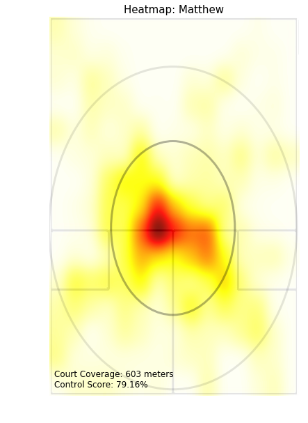
This heatmap can be used to assess the court control of a player. The basic strategy of squash is to stay as close to the center of the court as possible, as from there you can hit the most effective shots. To quantify how well a player has done this, I’ve awarded a player a point for each frame in the large ellipse, five points for each frame in the small ellipse, and deducted five points for each frame outside both ellipses. The “Control Score” represents the ratio of total points earned to number of points if all frames were in the small ellipse. I tinkered with the weights of these points until I got to a point where I was comfortable with how different matches showed relative percentages, but going forward I would like to do some more testing to be able to use this as a predictive statistic.

With the timeline of the project, I was only really able to create heatmaps based on the data, but I think the next step would be to implement tracking of the ball and use that to analyze rally hit points and average pace of certain shots.

Takeaways

With this being my last Metis project, I think my big takeaway is how far I’ve come in my data science knowledge. Thinking back to when I erroneously invoked NLP in an interview four months ago despite not really understanding how it worked, I never could’ve imagined I could do a project like this. It was a lot of fun to work on a project that I designed entirely by myself, and very satisfying to finish ahead of time. I hope to keep up my data science learning after Metis, even while I search for a job.